When working with charts that support displaying a timeline (usually a Temporal Evolution Chart with an attribute byTime set to true), the x-axis can be customised to display the level of details that suits you best. The following attributes can be used:

You can display future or past versions on a chart using the forecast element on a measure, as shown below.

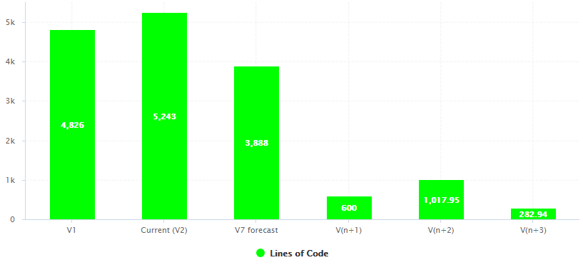
Planned (future) versions on a Temporal Evolution Chart

<chart type="TemporalEvolution" renderer="BAR" id="TE_BAR_FORECAST">
	<measure color="GREEN" label="Lines of Code">LC
		<forecast>
			<version value="SLOC" timeValue="DATE(2016,06,30)" label="V7 forecast" />
			<version value="600" timeValue="DATE(2016,07,31)" />
			<estimatedVersion timeValue="DATE(2016,08,31)" />
			<estimatedVersion timeValue="DATE(2016,09,30)" />
		</forecast>
	</measure>
</chart>

The forecast points on the chart can be:

The forecast element accepts the following attributes:

When using forecast with dynamically estimated future values, use the estimatedVersion element with the following attributes:

When using forecast with hard coded values for, use the version element with the following attributes:

Tip

Displaying estimates for dynamically for the next 6 months is more efficient with chart where values are plotted according to when they were created on a time axis (see the section called “Time Axis Configuration”) and can be done as shown in the following example:

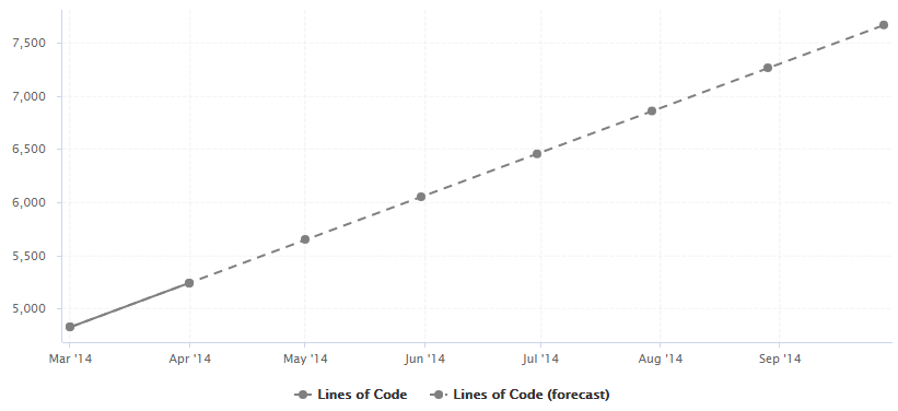
A rolling 6-month projection chart

<chart type="TE" byTime="true" id="FORECAST_ROLLING_EXAMPLE">
	<measure label="Lines of Code" color="GRAY">LC</measure>
	<measure stroke="DOTTED" label="Lines of Code (forecast)" color="GRAY">LC
		<forecast>
			<estimatedVersion timeValue="CURRENT_VERSION_DATE+DAYS(30)"  />
			<estimatedVersion timeValue="CURRENT_VERSION_DATE+DAYS(60)"  />
			<estimatedVersion timeValue="CURRENT_VERSION_DATE+DAYS(90)"  />
			<estimatedVersion timeValue="CURRENT_VERSION_DATE+DAYS(120)" />
			<estimatedVersion timeValue="CURRENT_VERSION_DATE+DAYS(150)" />
			<estimatedVersion timeValue="CURRENT_VERSION_DATE+DAYS(180)" />
		</forecast>
	</measure>
</chart>

CURRENT_VERSION_DATE is a metric defined in the analysis model as follows:

<Measure measureId="CURRENT_VERSION_DATE" defaultValue="-1">
	<Computation targetArtefactTypes="PACKAGES;FILE" result="VERSION_DATE()" />
</Measure>

On a Temporal Evolution Chart, you can render goals graphically by defining a starting point, an end date and a value you want to reach. This is done using the goal element on your chart, and replaces the deprecated Temporal Evolution Line With Goal and Temporal Evolution Bar With Goal charts.

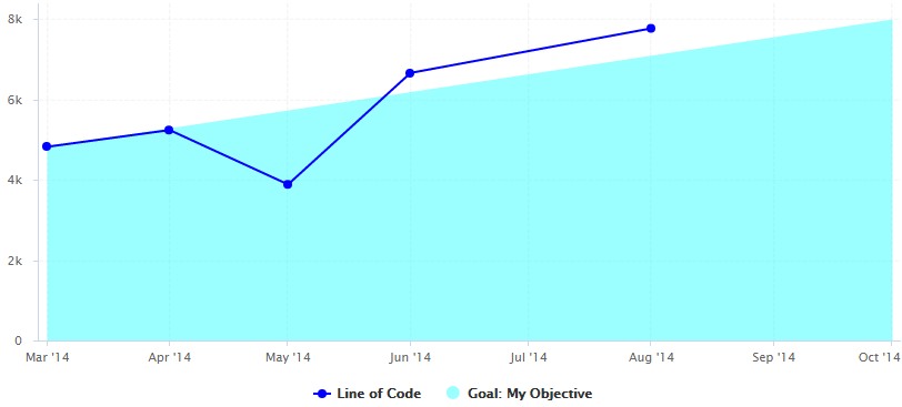
A Temporal Evolution Chart with an area that represents the goal for the metric LC

<chart type="TE" id="GOAL_EXAMPLE" byTime="true">
	<dataset renderer="AREA">
		<goal color="CYAN" alpha="100" label="My Objective">
			<forecast>
				<firstMeasureVersion id="LC" />
				<version value="8000" timeValue="DATE(2014,10,01)" />
			</forecast>
		</goal>
	</dataset>
	<dataset renderer="LINE">
		<measure color="BLUE" label="Line of Code">LC
			<forecast>
				<version value="SLOC" timeValue="DATE(2014,05,01)" label="V3" />
				<version value="6666" timeValue="DATE(2014,06,01)" />
				<version value="3333+4444" timeValue="DATE(2014,08,01)" />
			</forecast>
		</measure>
	</dataset>
</chart>

In the example above, the first dataset (rendered as an AREA ) is used for the goal, while the second (rendered as a LINE ) is used for the display of the LC metric.

The goal element supports the color , label and alpha attributes as they are described in the section called “Common Attributes for measure and indicator ”. It accepts a child forecast element with one or more traditional version elements (as described in the section called “Displaying Planned Versions”), as well as an optional firstMeasureVersion attribute that will define the starting point to draw the goal. In the example above, the goal is rendered the first time that the metric LC has a value and is drawn using the value of this metric at this point in time. The goal to reach is hard-coded to 8000 on October 1st 2014, but you could use any metrics from you model to generate dynamic values.

Tip

Using goals, you can easily draw burn down charts for you agile projects.

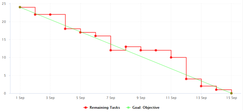
A burn down chart of remaining tasks in a sprint

<chart type="TE" id="BURN_DOWN_CHART" byTime="TRUE" timeInterval="DAY">
	<dataset renderer="STEP">
		<measure color="RED" alpha="200" label="Remaining Tasks">NUM_TASKS</measure>
	</dataset>
	<dataset renderer="LINE">
		<goal color="GREEN" alpha="100" label="Objective">
			<forecast>
				<firstMeasureVersion id="NUM_TASKS" />
				<version value="0" timeValue="SPRINT_START + DAYS(C.SPRINT_LENGTH)" />
			</forecast>
		</goal>
	</dataset>
</chart>

In this example, we start drawing the diagonal when NUM_TASKS first has a value for the project, and set the objective to reach zero by dynamically computing the end of the sprint based on the sprint start date and a constant that defines the sprint length.